Welcome to Kalman Filter Section

Task 1

Estimate drag and momentum

To build the state space model for your system, you will need to estimate the drag and momentum terms for your A and B matrices. Here, we will do this using a step response. Drive the car towards a wall at a constant imput motor speed while logging motor input values and ToF sensor output.

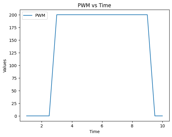
First I choose my step response from 0 to 200 PWM (maximum PWM in Lab 5 : PID controller) at 0.5s. The corresponding figure is shown below: (the unit of x-axis is 0.2s, means that when x is 10, the actual time is 10*0.2 = 2s)

As you can see, the PWM start to rise at about 2.5*0.2 = 0.5s

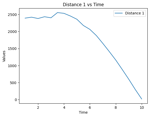
Then I get the data sending from the car, and ploted the distance from TOF sensor as below:(the unit of x-axis is 0.2s, means that when x is 10, the actual time is 10*0.2 = 2s)

As shown in the figure above, the car is driving towards to the wall and get the steady speed after 6*0.2 = 1.2s.

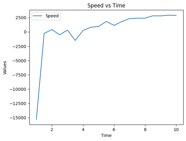
To have a more direct spot on whether the car reaches a steady speed, I plotted the figure that Speed vs. Time: (the unit of x-axis is 0.2s, means that when x is 10, the actual time is 10*0.2 = 2s)

From the figure of the speed, we could know the car reaches the steady speed after 8*0.2 = 1.6 seconds, so I printed out the speed value to get a more precise speed:

From the data shown above, we finally calculated the steady speed as 2750 mm/s.

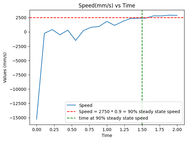
The we calculated the 90% rise time using the figure below:

The figure above illustrates that the car reaches the 90% steady speed at 1.5s, so that the overall rise time is 90%_speed_time - start_time = 1.5-0.5 = 1s

Task 2

Calculate mass and drag

Here below shows the formulars and results I used to calculate the mass and drag:

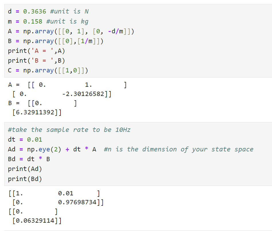
Then I used these parameters to designed the A, B and C matrix:

Task 3

Kalman Filter

Firstly I stored the data from lab 5 in a csv file using the code below:

                            
    import csv
    import numpy as np
    
    # File paths
    time_file = 'time_values.csv'
    distance_file = 'distance_values.csv'
    speed_file = 'speed_values.csv'
    ispeed_file = 'ispeed_values.csv'
    
    # Writing data to CSV files
    with open(time_file, 'w', newline='') as csvfile:
        writer = csv.writer(csvfile)
        writer.writerow(time_values)
    
    with open(distance_file, 'w', newline='') as csvfile:
        writer = csv.writer(csvfile)
        writer.writerow(distance1_values)
    
    with open(speed_file, 'w', newline='') as csvfile:
        writer = csv.writer(csvfile)
        writer.writerow(speed_values)
    
    with open(ispeed_file, 'w', newline='') as csvfile:
        writer = csv.writer(csvfile)
        writer.writerow(ispeed_values)
                            
                            

Then I used these code to read data from CSV file:

                            
    import csv
    import numpy as np
    
    # File paths
    time_file = 'time_values.csv'
    distance_file = 'distance_values.csv'
    speed_file = 'speed_values.csv'
    ispeed_file = 'ispeed_values.csv'
    
    # Reading data from CSV files
    time_values = np.genfromtxt(time_file, delimiter=',')
    distance1_values = np.genfromtxt(distance_file, delimiter=',')
    speed_values = np.genfromtxt(speed_file, delimiter=',')
    ispeed_values = np.genfromtxt(ispeed_file, delimiter=',')
                            
                            

Then I implemented the Kalman filter, the code is shown below (well-annotated):

                            
    #store the final calculated kalman filtered distance
    kfdistance = []
    
    def kf(mu,sigma,u,y):
        #mu is current state
        #sigma is uncertainty in current state
        #u is speed
        #y is TOF reading
        mu_p = Ad.dot(mu) + Bd.dot(u)   #mu_p = Ad*mu + Bd*u
        sigma_p = Ad.dot(sigma.dot(Ad.transpose())) + sig_u
        
        
        sigma_m = C.dot(sigma_p.dot(C.transpose())) + sig_z
        #calculate kalman gain
        kkf_gain = sigma_p.dot(C.transpose().dot(np.linalg.inv(sigma_m)))
        y_m = y-C.dot(mu_p)
    
        #update state and new uncertainty in state
        mu = mu_p + kkf_gain.dot(y_m)    
        sigma=(np.eye(2)-kkf_gain.dot(C)).dot(sigma_p)
            
        return mu,sigma
    
    
    #initial state
    x = np.array([[distance1_values[0]],[0]])
    #initial state uncertainty
    sigma = np.array([[1^2, 0] ,[0, 20^2]])
    
    #Model uncertainty
    sigma_1 = 4
    sigma_2 = 5
    
    #sensor uncertainty
    sigma_3 = 10
    
    #confidence in state
    sig_u = np.array([[sigma_1**2,0],[0,sigma_2**2]]) ##We assume uncorrelated noise, and therefore a diagonal matrix works. 
    # confidence in sensor measurement
    sig_z = np.array([[sigma_3**2]]) 
    
    
    #apply Kalman Filter for each step in time
    for i in range(len(time_values)):
        x, sigma = kf(x, sigma, 65/65, distance1_values[i])
        kfdistance.append(x[0])
    
    
    plt.plot(time_values, kfdistance, label = 'kfdistance')
    plt.scatter(time_values, kfdistance)
    plt.plot(time_values, distance1_values, label = 'TOF')
    plt.scatter(time_values, distance1_values)
    plt.title('Distance')
    plt.xlabel('Time')
    plt.ylabel('Distance(mm) or speed (mm/s)')
    plt.legend()
    plt.show ()
                            
                            

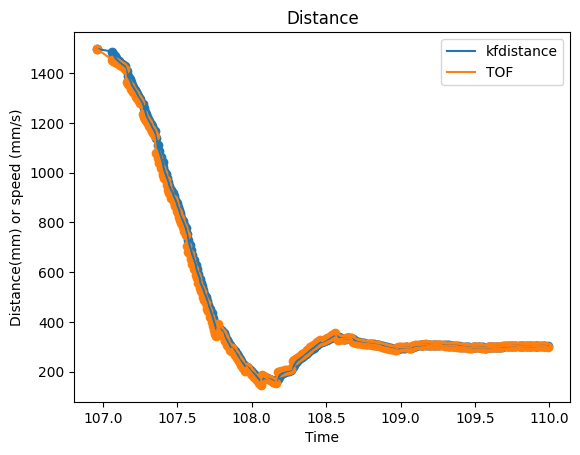
Here below shows the final results.

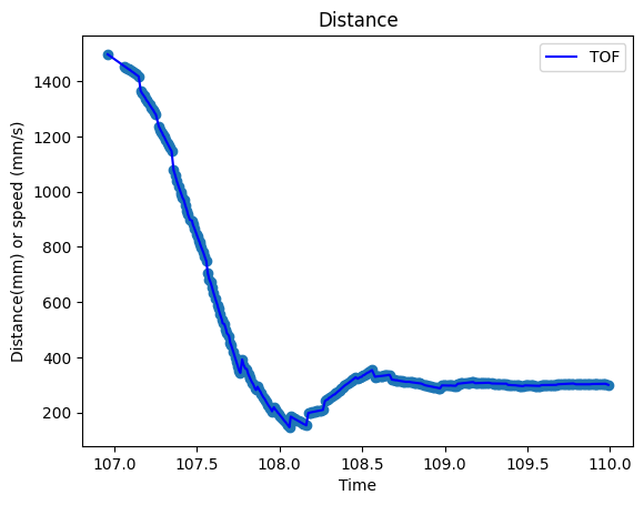
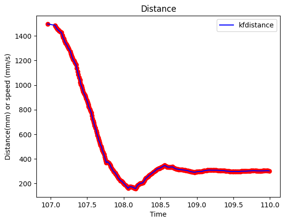
The two results overlaps well, so let us compare them seperately:

As shown below the distance calculated by kalman filter is also precises but much smoother than that of TOF.